A free surface moves under the traction it carries. That makes the wall-normal stress the quantity driving the model rather than something read off at the end, and it is the reason we went back to how the boundary condition underneath it is imposed.
The condition itself is ordinary. Free slip is no flow through the boundary and no tangential drag along it,
On a box the first of those is a single velocity component. You hold on a vertical wall, the solver removes a row, and there is nothing further to discuss. On a sphere, an annulus, a mesh that has been moved, or a surface with topography, is not a component of anything. That is the whole difficulty, and everything below is a way around it.
The second condition is worth naming because it is the one people forget. Zero tangential traction is natural: it is what you get by leaving the boundary term out of the weak form. Nothing has to be done to impose it, and something has to be done to avoid imposing it accidentally.
Where the boundary term comes from
Every method below is a statement about one term. Multiplying the momentum balance by a test function and integrating by parts gives
Drop the surface integral and you have imposed zero traction in both directions — free everything, not free slip. Free slip keeps the tangential half of that and replaces the normal half with the constraint. How you do the replacing is the choice.
Four ways, in order
They fall into two pairs, and the pairing is the useful way to hold them. Two impose the constraint weakly, by adding a term to the momentum equation and letting the solution satisfy the condition to within the accuracy of that term: a direct penalty, and Nitsche’s method, which differ in whether the term is consistent. Two impose it exactly: by construction, changing the basis so that the constraint is a component that can be struck out, or by a Lagrange multiplier, adding an equation that enforces it. The weak pair have a parameter to choose and a floor they cannot go below. The exact pair have neither, and both return the boundary traction as part of the answer.
A direct penalty
Add a term that punishes any flow through the boundary:
One line, no new machinery, and it works on any geometry. It is still in a good many working scripts, and deservedly. What you are solving is a perturbed problem, though, and it is perturbed by exactly the amount the constraint is violated: the discrete solution sits where the penalty term balances the traction it is fighting, which leaves small but not zero. Making it smaller means pushing harder, and pushing harder conditions the operator worse. The error is traded against the conditioning, and measured below, that trade runs out: past 104 the leak stops improving, and by 106 the solve fails. Nitsche moves the floor down rather than removing it — it fails too, at its own threshold.
Underworld spells it as a boundary traction opposing normal flow, using the facet normal at the quadrature points:
G = mesh.Gamma
stokes.add_natural_bc(1.0e4 * G.dot(v.sym) * G, "Upper")Nitsche
The reason the penalty is only accurate in the limit is that it is not consistent: substituting the true solution does not leave the equation satisfied, because the true solution is subject to a boundary traction the penalty form ignores. Nitsche’s method 1 restores consistency by carrying that traction explicitly:
The first of the three is the consistency term: it is the boundary traction the integration by parts produced, and putting it back is what makes the true solution satisfy the discrete equations exactly. The second is its transpose, which keeps the form symmetric and buys optimal convergence in . The third is the penalty again, and it is still needed — but now for stability rather than for accuracy, and has a threshold set by an inverse inequality rather than being a dial you turn up until the answer looks right.
This is a real improvement and it is still a weak imposition. The constraint holds to the accuracy of the discretisation, not to the accuracy of the arithmetic — measured below, it leaks a few parts in a thousand on a mesh of the resolution people actually run, and the leak falls with the mesh rather than with the machine.
A constraint equation, with a multiplier
The two above add a term to an equation. This one adds an equation.
Carry a scalar field on the boundary and require, as a row of the system in its own right,
with entering the momentum row as the traction that holds the constraint. It is a Lagrange multiplier, and the system becomes a larger saddle point: velocity, pressure, and now .
The constraint row is exact, so unlike a penalty there is no parameter whose size decides how well it holds. Two practical things do have to be dealt with.
is carried as a full-domain field but only its boundary trace means anything, so the interior degrees of freedom are constrained out of the global system in the section before the solve sees it. They are not solved for and they do not enlarge the block. The interior rows are the screening block alone, so the interior multiplier is determined by the boundary trace and carries no independent signal.
The Schur complement is poorly conditioned on its own, so an augmented-Lagrangian term is added to the momentum row. It does not change what the constraint enforces, because the row still carries the exact constraint. It does change what is, which is the subject of a section below.
stokes = uw.systems.Stokes_Constrained(mesh, velocityField=v, pressureField=p)
h = stokes.add_constraint_bc(0.0, "Upper")
stokes.solve()
And the reason to care about it beyond the constraint: at convergence the
momentum row’s boundary term is the normal traction. It is not recovered from
the velocity field afterwards — it is an unknown the solve returned, available
through traction and, divided by , through topography.
That term is the whole boundary load, , and not the multiplier alone. The second part vanishes only where the constraint row is satisfied exactly; discretely it is satisfied to the solver’s tolerance and multiplies that residual back into the traction. With a viscosity-weighted and a lateral viscosity contrast it is most of the answer, so the two parts are not separable in practice — which is the first hint that this traction and the rotated constraint’s reaction are the same object.
Rotating the degrees of freedom
Stop asking for the constraint and impose it. At each constrained node, change the basis in which the velocity unknowns are expressed, from the global Cartesian frame to the local frame. In that basis “no flow through the boundary” is again a single component, and it is removed the same way it would be on a box.
Collect the per-node rotations into a block-diagonal , equal to the identity at every node that is not constrained. The rotated system is
and the wall-normal row of is struck out. The constraint then holds to machine precision, because it is not being solved for at all.
This is the classical answer, not a new one. It is in the early finite-element literature, and Engelman et al. (1982) were already reviewing the alternatives and choosing between them on grounds of global mass conservation in 1982. What is worth explaining is not the idea but why, given that it is exact and the others are not, it is the least used of the three.
What it costs, and the cost is structural
Rotating the degrees of freedom leaves the discrete problem in a mixed basis. Interior nodes hold ; constrained nodes hold . Nothing about that is difficult in itself, and everything downstream has to agree about which nodes are which.
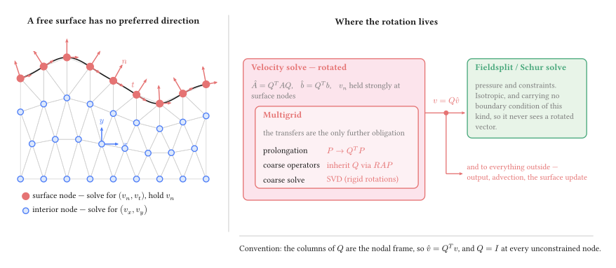
Where the rotation lives. The obligation is contained: the velocity solve is rotated and carries its multigrid with it, while the Schur complement and the pressure solve beside it never handle a rotated vector, because the pressure block carries no boundary condition of this kind. One un-rotation sits on the boundary between them and feeds both.
Four things carry : the operator, the right-hand side, the solution on the way out, and the multigrid prolongation. The coarse operators inherit it through the Galerkin triple product rather than being rotated separately, and the coarse solve then has to be an SVD, because a Galerkin-coarsened rotated operator inherits the rigid-rotation null space of the constrained problem and a redundant LU factorisation meets a zero pivot in it.
That last point is worth dwelling on, because it is the one that surprises. The constraint never has to be re-imposed on a coarse mesh — which is fortunate, since we install no discretisation there and could not impose it if we wanted to. It arrives anyway, algebraically, through with a rotated . The evidence that it really arrives is that the coarse operator inherits the null space, which is a property only the constrained problem has.
None of this is an argument against the method. It is an argument for knowing what is being taken on, and it is the honest reason a weakly imposed condition survives in codes that could do this instead.
Which normal
A question with a less obvious answer than it looks, and the measurements further down say it is the most consequential choice in the note. The boundary of a discretised domain is a set of straight facets, and the assembled constraint is an integral over those facets. The node normal consistent with that integral is the average of the adjacent facet normals weighted by facet measure — not the normal of the smooth surface the mesh approximates, and not the facet normal on its own.
This is the consistent normal of Engelman et al. (1982), and we should say so plainly: we re-derived it from the assembled boundary integral, and Engelman, Sani and Gresho derived it in 1982 from global conservation of mass, which is the same object arrived at from the other side. Their paper is about exactly this — how to impose a normal or tangential condition on a boundary that does not line up with the coordinate directions — and the recommendation is the one here.
Using the analytic normal is exact for the geometry and therefore inconsistent with the discretisation, which is the wrong way round: the solver is not solving on the sphere, it is solving on the polyhedron. Using the facet normal is consistent with each facet separately and over-constrains the nodes between them, which is the failure measured in “A constraint that is satisfied, and wrong” below. In parallel the same argument has a sharper edge, because a normal accumulated rank-locally is wrong at a partition boundary, where a node’s facets are split across ranks and no rank sees them all.
The consistent normal is not the end of the matter. Behr (2004) takes it as the starting point — “preferred from the point of view of conservation” — and reports that in sloshing problems it still does not guarantee a good discrete slip condition, with non-physical recirculation appearing at curved walls; the remedies offered there are the Navier slip condition and a “BC-free” boundary. We have read the abstract rather than the paper, and have not looked for that recirculation in our own cases. It is the obvious thing to test next for anyone running free slip on a strongly curved wall.
The option this note leaves out
Solving in spherical or cylindrical components makes the wall-normal direction a coordinate direction again, and the constraint returns to being “hold one component”. That is the same rotation as above, applied once for the whole domain instead of node by node, and applied that way it costs nothing structurally: there is no mixed basis, because every node is in the same basis.
It works exactly when the boundary lies along a coordinate surface. A sphere, an annulus, a cylinder. It does nothing for topography, for a mesh that has been deformed, or for a tilted internal surface, which is the general case this note is about. The per-node rotation is what remains once the geometry stops cooperating, and its structural price is what buys the generality.
When the choice matters
Here is the awkward part. Solve a convection model with any of these and the velocity field is the same to plotting accuracy, as long as each is set up properly. A leak of order 10-3 in is invisible to anything that consumes the velocity, and consuming the velocity is most of what a model does. If that is your situation, use the simplest thing that works — and read the section on which normal before you do, because that is the choice that can spoil the velocity as well.
The difference appears when the wall-normal traction is the answer rather than a by-product: dynamic topography, a plate-boundary force balance, anything compared against a geoid or a gravity field. That is what the two sections after the leak measure, against an exact surface stress, and the answer is not the one we expected. The treatments that impose the constraint properly all recover the same surface stress at a given mesh, because the recovery sets the floor rather than the boundary condition; what the rotated constraint buys is a route to the traction that does not go through a recovery at all, and it is three times better on the same solve.
Under the rotated constraint the reaction is : it is the
multiplier the solve has already computed, and it comes out of
boundary_normal_traction without differentiating the answer.
The leak, measured
An annulus, no slip on the inner radius, the treatment under test on the outer, driven by a degree-four radial density anomaly. The number is the largest normal velocity on the outer boundary, taken against the true radial direction and divided by the flow speed: the fraction of the flow going through a boundary nothing should pass through. Penalty at 104, Nitsche at .
The penalty appears twice, because the normal it is written against turns out
to matter more than the method it is written into. One column uses the
quadrature-point facet normal mesh.Gamma, which is the documented form; the
other uses the measure-weighted node normal mesh.boundary_normal, which is
what Nitsche and the rotated constraint use by default.
| cell size | penalty, facet normal | penalty, node normal | Nitsche | multiplier | rotated |
|---|---|---|---|---|---|
| 0.150 | 4.5 × 10⁻³ | 3.3 × 10⁻³ | 4.6 × 10⁻³ | 8.3 × 10⁻⁴ | 7.3 × 10⁻¹¹ |
| 0.100 | 2.5 × 10⁻³ | 2.7 × 10⁻³ | 2.2 × 10⁻³ | 1.6 × 10⁻⁴ | 6.5 × 10⁻¹¹ |
| 0.075 | 8.5 × 10⁻⁴ | 2.6 × 10⁻³ | 1.7 × 10⁻³ | 5.6 × 10⁻⁵ | 1.0 × 10⁻¹⁰ |
| 0.050 | 9.5 × 10⁻⁴ | 2.6 × 10⁻³ | 5.8 × 10⁻⁴ | 1.2 × 10⁻⁵ | 8.4 × 10⁻¹¹ |
Nitsche leaks parts in a thousand and improves roughly as — the rate consistency buys. The multiplier starts an order of magnitude better and falls much faster, near , because the constraint row is an equation rather than a term whose weight has to be chosen. The rotated constraint does not move at all: it sits at the solver’s floor at every resolution, because the mesh has nothing to do with it. The penalty against the node normal does not improve with the mesh either, and for the opposite reason: at a fixed coefficient its leak is set by the coefficient.
The control matters more than the result. With the outer boundary left free the same measurement reads 0.98 — nearly all the boundary flow is normal — so the metric can see a leak when there is one.
The first column is the one to be careful with. Its leak falls with the mesh, which reads as the method working, and it is not: the surface stress measured further down says that solve is 60% wrong in the velocity and 26% wrong in the stress, and refining it does not help. The leak is small because the boundary is being frozen. A metric that only asks whether the constraint is satisfied cannot tell those apart.
What each parameter buys
The two weak methods look alike in that table. They are not alike, and their own parameters are what tells them apart.
| penalty, facet | leak | penalty, node | leak | (Nitsche) | leak | ||
|---|---|---|---|---|---|---|---|
| 10² | 2.6 × 10⁻¹ | 10² | 2.6 × 10⁻¹ | 1 | diverged | ||
| 10³ | 2.3 × 10⁻² | 10³ | 2.6 × 10⁻² | 10 | 1.7 × 10⁻³ | ||
| 10⁴ | 8.5 × 10⁻⁴ | 10⁴ | 2.6 × 10⁻³ | 100 | 2.7 × 10⁻⁴ | ||
| 10⁵ | 9.6 × 10⁻⁴ | 10⁵ | 3.0 × 10⁻⁴ | 1000 | 3.0 × 10⁻⁵ | ||
| 10⁶ | diverged | 10⁶ | 4.5 × 10⁻⁵ | 10⁴ and above | diverged |
Nitsche is bounded at both ends. Below the form is no longer coercive and no amount of tuning recovers it; from in this problem the line search stops converging. The virtue of is that it sits in the middle of that window on any mesh, because is dimensionless and the term it scales already carries . The penalty coefficient carries no such scaling, which is why the value that works is a property of the problem rather than a default — and, on the second half of this note’s test, of the local viscosity as well.
The two penalty columns are the same method against different normals, and they behave differently in a way the leak alone does not explain. Against the node normal the leak keeps falling, a decade of coefficient for a decade of leak, all the way to 106. Against the facet normal it stops improving after 104 and the solve fails at 106. That looks like the conditioning wall a penalty is expected to have. It is not: what stalls is the leak, because by 104 the boundary is nearly frozen and there is little normal flow left to remove. The stress section below measures the same runs against an exact answer, and they are getting worse throughout.
The stress, measured
The leak says how well each treatment holds the boundary. Whether the answer is right is a different question, and it needs an exact answer to compare against.
Kramer, Davies and Wilson 4 give exact Stokes
solutions in a cylindrical annulus, and their assess package publishes the
radial stress itself rather than leaving it to be recovered from a velocity
field. Underworld wraps it as uw.analytic.CylindricalStokes. The case here is
the smooth one: a density anomaly with and
, viscosity 1, free slip on both radii. On the outer boundary the exact
radial stress is a single harmonic,
fitted to a residual of 10-16, so the whole of the surface stress is that one amplitude and the metric is its relative error.
The inner boundary carries the exact velocity as a Dirichlet condition instead of a free-slip treatment of its own. The exact solution satisfies both, so the problem is unchanged, and the treatment under test is then the only free-slip condition in the model.
There are two routes to the surface stress and the difference between them is the point of the section:
recovered — project out of the solved velocity and pressure. Every treatment can do this, and it is the only route the weak ones have.
reaction —
boundary_normal_tractionfor the rotated constraint, and the multiplier field for the constraint method. Not recovered from the solution: an unknown the solve returned.
Both are taken against the true radial direction, which is also the direction
the oracle publishes, so no treatment is scored against its own normal. The
reaction and the multiplier come back with the opposite sign to —
they are the traction holding the boundary rather than the traction the fluid
exerts, and dynamic_topography carries the sign back — so amplitudes are
compared unsigned.
| cell size | penalty, facet | penalty, node | Nitsche | constraint | rotated | rotated, reaction | multiplier field |
|---|---|---|---|---|---|---|---|
| 0.150 | 1.5 × 10⁻¹ | 2.5 × 10⁻² | 5.9 × 10⁻² | 2.4 × 10⁻² | 2.4 × 10⁻² | 6.8 × 10⁻³ | 8.6 × 10⁻³ |
| 0.100 | 1.3 × 10⁻¹ | 1.1 × 10⁻² | 2.4 × 10⁻² | 1.0 × 10⁻² | 1.0 × 10⁻² | 3.3 × 10⁻³ | 8.5 × 10⁻⁴ |
| 0.075 | 1.1 × 10⁻¹ | 7.2 × 10⁻³ | 1.5 × 10⁻² | 6.3 × 10⁻³ | 6.2 × 10⁻³ | 2.1 × 10⁻³ | 1.7 × 10⁻³ |
| 0.050 | 6.3 × 10⁻² | 3.6 × 10⁻³ | 6.3 × 10⁻³ | 2.7 × 10⁻³ | 2.7 × 10⁻³ | 1.1 × 10⁻³ | 1.4 × 10⁻³ |
The first five columns are all the recovered stress, so they differ only by which boundary condition produced the field. The last two are the reaction and the multiplier on the same solves. Penalties at 104, Nitsche at , which are the values the leak table used. With the outer boundary left free the same measurement reads 1.0 — the surface stress is gone — so the metric can see the condition being removed.
Once the constraint is imposed against the node normal, which treatment imposed it stops mattering to the recovered stress. At cell 0.075 the rotated constraint gives 6.2 × 10⁻³, the multiplier 6.3 × 10⁻³, the penalty at 105 6.3 × 10⁻³ and Nitsche at 6.6 × 10⁻³. Those are the same number. What sets it is the recovery — a projection of a stress differentiated out of a piecewise-quadratic velocity — and not the boundary condition underneath. The reasoning this note began with — that a traction recovered from an approximate constraint inherits the approximation — is not what the measurement shows once the constraint is written against the right normal. It shows a floor that all of them share.
The reaction is about three times better than the recovery, on the same solve. 2.1 × 10⁻³ against 6.2 × 10⁻³ at cell 0.075, and it converges at the same rate rather than a better one. It costs nothing — it is the residual the solve has already assembled, and no field is differentiated to get it — and the timings below put a number on “nothing”.
The multiplier’s traction is the same story from the other side, and lands in the same place: 8.5 × 10⁻⁴ to 1.7 × 10⁻³ over the three finer meshes. Its column does not fall smoothly with , because part of what it reports is the augmentation times the constraint residual, and how far a particular solve drove that residual is not a function of the mesh.
The parameter that was enough for the leak is not enough for the stress. Nitsche at leaks 1.2 × 10⁻³ in this problem and gets the stress amplitude 1.5% wrong. At the leak improves by a factor of nearly forty and the stress by a factor of two, to the recovery floor, where more buys nothing. Reading the leak alone would have said was converged.
A constraint that is satisfied, and wrong
The facet-normal penalty column does not converge. That is not a slow rate; the error grows slightly as the mesh is refined, and the leak is excellent throughout.
| cell size | leak | velocity error | stress error |
|---|---|---|---|
| 0.150 | 8.9 × 10⁻⁶ | 0.60 | 0.21 |
| 0.100 | 8.2 × 10⁻⁶ | 0.61 | 0.24 |
| 0.075 | 1.1 × 10⁻⁵ | 0.61 | 0.25 |
| 0.050 | 1.9 × 10⁻⁵ | 0.60 | 0.26 |
| 0.035 | 2.3 × 10⁻⁵ | 0.59 | 0.26 |
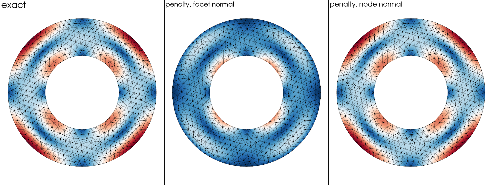
The same problem, the same coefficient of 106, the same colour scale, and the only difference between the middle and right panels is which normal the penalty is written against. Against the facet normal the flow along the outer boundary is suppressed: the peak speed falls by a quarter and the two fast lobes at the boundary are gone. Refining the mesh does not bring them back.
The coefficient is 106 and the normal is mesh.Gamma, the facet normal at
the quadrature points. The same coefficient against the measure-weighted node
normal, on the same meshes, gives velocity errors of 1.0 × 10⁻², 2.4 × 10⁻³,
1.0 × 10⁻³ and 4.9 × 10⁻⁴ and stress errors of 2.4 × 10⁻², 6.3 × 10⁻³,
2.7 × 10⁻³ and 1.4 × 10⁻³. One difference, one line of code, and one method
converges while the other does not.
The mechanism is old and well understood. Imposing facet by facet asks a node shared by two facets to satisfy two different constraints, and two independent constraints on a two-component velocity leave nothing. Push the coefficient up and the vertex velocities go to zero: the flow is being asked to stay inside a polygon rather than a circle, and the polygon is not a good enough approximation of the circle for that particular question. The discrete limit is a different problem from the smooth one, so refining the mesh does not approach the smooth answer.
Two things follow for practice. A direct penalty is a perfectly good method, but it has to be written against the node normal. And the leak is not a sufficient check: at a coefficient of 103 the facet-normal penalty leaks 3 × 10⁻² and gets the stress amplitude right to 1.9 × 10⁻³, while at 108 it leaks 1 × 10⁻⁷ and is 26% wrong. Over that range the constraint improves by five orders of magnitude and the answer gets steadily worse.
The multiplier and the consistent boundary flux are the same object
The correction above is not a patch. Write the momentum row’s boundary term out and the identity is immediate: the assembled load is , and at convergence it balances the volume residual restricted to the boundary, which is precisely the nodal load the consistent boundary flux back-calculation reads 5. So
the CBF traction de-smeared with the boundary mass. The multiplier is not a second, independent estimate of the surface stress: it is the same computation the rotated constraint’s reaction performs, arrived at by carrying the traction as an unknown instead of reading it out of the residual afterwards. Dropping the term is dropping part of the load, which is why it fails exactly where is large.
Measured across the two solves — they are different discrete problems, so this is agreement rather than an identity check — the corrected multiplier and the rotated reaction differ by 3.2% at a contrast of 100 and 4.9% at 106, both inside each route’s own error against the exact answer (5 to 9%). The identity also says why the two cannot be read off a single solve. On a multiplier-constrained boundary the constraint enters the row it constrains, so the assembled residual there is balanced at convergence and the back-calculation reads zero — measured, rms 4 × 10⁻¹³ against a traction of 0.37. There is no reaction left in the residual because the multiplier is holding it. The two routes are alternatives, not a cross-check available at the same time.
This also settles a question the free-surface work left open. That work used SolCx the same way, to choose among topography recoveries, and landed on a rotated free-slip lid with the CBF reaction and a continuous pressure — corr 0.999, relative 0.04 — while rejecting the multiplier. Both conclusions were right about what was in front of them: the multiplier as returned is missing the augmentation share, and the CBF reaction is the same quantity with nothing missing.
The other half: a lateral viscosity contrast
No exact solution has both a curved boundary and a laterally varying viscosity,
so the case where weak constraints are most often reported to give trouble is a
separate test with a trivial geometry. SolCx is that test: the unit box, free
slip on all four walls, viscosity 1 to the left of and to the
right. uw.analytic.SolCx publishes the exact dynamic topography on the top
wall. Three walls carry the ordinary component condition and the treatment under
test is on the top wall alone.
On a box every treatment reduces to holding one velocity component, so nothing here is about normals. What it can say is whether a treatment holds the traction it was given when the viscosity beside it jumps.
Relative error of the surface topography along the top wall, mean removed, at 32 × 32 elements. Each entry is the whole wall and then the wall with two elements trimmed from each end.
| component Dirichlet | penalty, 104 | multiplier | rotated | |
|---|---|---|---|---|
| 10 | 0.048 / 0.054 | 0.045 / 0.051 | 0.048 / 0.054 | 0.048 / 0.054 |
| 10² | 0.072 / 0.081 | 0.056 / 0.060 | 0.072 / 0.081 | 0.072 / 0.081 |
| 10³ | 0.075 / 0.084 | 0.234 / 0.230 | 0.075 / 0.084 | 0.075 / 0.084 |
| 10⁴ | 0.076 / 0.085 | 0.698 / 0.697 | 0.076 / 0.085 | 0.076 / 0.085 |
| 10⁶ | 0.076 / 0.085 | 0.992 / 1.000 | 0.075 / 0.084 | 0.076 / 0.085 |
The three exact treatments agree to three figures at every contrast, whole wall and trimmed alike. That is the result to take from this half, and it took two fixes to get: the multiplier had to report the whole traction rather than , and the rotated constraint had to hold the corner where it meets the side walls. Before them the rotated column read 0.322 at a contrast of 10 — six times the reference, all of it two nodes — and the multiplier column was an order of magnitude out at 106.
Read the first column as the floor. The component Dirichlet condition is exact and has no parameter, and its velocity error is 8.8 × 10⁻⁶ at a contrast of 106. It still reads 0.085. That number is the recovery’s error, not a boundary condition’s: on the stiff half the recovered is a difference between the pressure and with , so a relative velocity error of 10-5 arrives in the stress at the size of the signal. Nothing here is worse than the reference except the penalty.
A bare penalty coefficient cannot serve both halves. At 104 it is the best
column in the table at low contrast — the constraint is weak enough not to fight
the recovery — and by 106 it is useless: 0.992, which is to say the recovered
topography carries none of the signal. Scaling the coefficient by the local
viscosity is the obviously right thing to want, and it does not solve here at any
magnitude we tried, from to (a Piecewise viscosity inside the
boundary term fails the line search). This is the same lesson as ’s window
on the annulus, in a place where the window closes entirely.
Nitsche is missing from this table, and honestly so. Our configuration of it on this box converges at a contrast of 106 and fails the line search at 10 — the opposite way round from every expectation — at 16 × 16 and 32 × 32 alike and at , 100 and 1000. Where it does converge, has to rise with the contrast exactly as the annulus said: at 106 and 16 × 16 the surface stress error is 25 at , 1.2 at 100 and 0.17 at 1000, while the constraint is held to 10-3 or better throughout. We are not confident enough in that configuration to put a column of numbers behind it.
What each one costs
Seconds on the annulus, uniform viscosity, one core, direct solver: the solve, and then the recovery of the surface traction by whatever route that treatment has. Median of three timed repeats after an untimed warm-up, run sequentially. The smaller meshes are here for the scaling; at ten thousand nodes the four treatments are separated by less than the run-to-run spread and only the largest row is worth reading.
| cell size | velocity nodes | penalty | Nitsche | multiplier | rotated |
|---|---|---|---|---|---|
| 0.050 | 4 802 | 0.03 / 0.073 | 0.03 / 0.060 | 0.04 / 0.002 | 0.03 / 0.004 |
| 0.030 | 12 852 | 0.08 / 0.128 | 0.08 / 0.131 | 0.12 / 0.005 | 0.07 / 0.007 |
| 0.020 | 28 338 | 0.18 / 0.257 | 0.18 / 0.268 | 0.26 / 0.011 | 0.17 / 0.010 |
| 0.013 | 71 424 | 0.45 / 0.626 | 0.47 / 0.652 | 0.67 / 0.027 | 0.43 / 0.016 |
Two things separate, and both are structural rather than incidental.
The multiplier’s solve costs about 50% more, consistently across the sweep — 0.67 s against 0.43 s at 71 000 nodes. That is the extra field and the larger saddle point. The other three are the same solve to within the spread; rotating the degrees of freedom costs nothing measurable here, because the rotation is a sparse orthogonal transform applied to a boundary’s worth of rows.
The recovery differs by a factor of 25 to 40, and it is the larger number. Projecting out of the solution is a second solve, and at every size in this table it costs more than the Stokes solve did — 0.63 s against 0.45 s at the largest. The two exact routes read their traction off the state the solve already returned: 27 ms for the multiplier, 16 ms for the rotated reaction. On a time-dependent model with a free surface that difference is paid at every step.
Which one to use
For a model that consumes the velocity and nothing else, all four are the same to plotting accuracy — provided the constraint is written against the node normal. That proviso is the only one that can spoil the velocity, and it costs one line.
When the wall-normal traction is the answer:
Rotated free slip is the default. It holds the constraint to machine precision rather than to the discretisation, its reaction is the most accurate surface stress measured here, and that reaction is nearly free. The price is structural — a mixed basis that the multigrid has to carry — and it is paid once, inside the solver, rather than by the person setting up the model.
The multiplier is its equal on accuracy and returns the same object by a different route; take it when you want the traction as an unknown of the system, or when the constrained problem’s conditioning suits you better. It costs about 50% more to solve.
Nitsche is the one to reach for when the boundary condition must change during the model — a wall that begins as a prescribed velocity and relaxes to a prescribed traction is a Nitsche problem, because a hard constraint cannot morph. Budget for tuning against the stress and not against the leak, and expect the window to move with the viscosity contrast.
A direct penalty is fine for a velocity-only model and needs the node normal, a coefficient chosen per problem, and a check on something physical before the answer is believed.
Using it
import underworld3 as uw

mesh = uw.meshing.Annulus(radiusInner=0.5, radiusOuter=1.0, cellSize=0.05)
stokes = uw.systems.Stokes(mesh)

# Value first: 0 is free slip. A non-zero scalar or expression prescribes the
# wall-normal datum u.n = u_n strongly instead.
stokes.add_rotated_freeslip_bc(0.0, "Upper")
stokes.add_rotated_freeslip_bc(0.0, "Lower")

stokes.solve()

# The constraint reaction, which is the boundary normal traction.
sigma_nn = stokes.boundary_normal_traction("Upper")
Leave the normal to Underworld unless the constraint has to follow the true
surface rather than the mesh. Passing an analytic normal — X / |X| on a
sphere — is exact for the geometry and keeps a consistency error against the
faceted assembly, which is usually not what you want.
Reach for Nitsche when the boundary condition has to change during the model. A hard constraint cannot morph: a wall that begins as a prescribed velocity and relaxes to a prescribed traction is a Nitsche problem, because the rotated constraint is either imposed or it is not.
- Nitsche, J. (1971). Über ein Variationsprinzip zur Lösung von Dirichlet-Problemen bei Verwendung von Teilräumen, die keinen Randbedingungen unterworfen sind. Abhandlungen Aus Dem Mathematischen Seminar Der Universität Hamburg, 36(1), 9–15. 10.1007/bf02995904
- Engelman, M. S., Sani, R. L., & Gresho, P. M. (1982). The implementation of normal and/or tangential boundary conditions in finite element codes for incompressible fluid flow. International Journal for Numerical Methods in Fluids, 2(3), 225–238. 10.1002/fld.1650020302
- Behr, M. (2004). On the application of slip boundary condition on curved boundaries. International Journal for Numerical Methods in Fluids, 45(1), 43–51. 10.1002/fld.663
- Kramer, S. C., Davies, D. R., & Wilson, C. R. (2021). Analytical solutions for mantle flow in cylindrical and spherical shells. Geoscientific Model Development, 14(4), 1899–1919. 10.5194/gmd-14-1899-2021
- Zhong, S., Gurnis, M., & Hulbert, G. (1993). Accurate determination of surface normal stress in viscous flow from a consistent boundary flux method. Physics of the Earth and Planetary Interiors, 78(1–2), 1–8. 10.1016/0031-9201(93)90078-n